All of these VB6 applications are available elsewhere but these examples are a little more detailed than some.
The file to download is either a self-extracting, .EXE file or a .ZIP file which will produce several files including a "ReadMe" text file, (which should be read!) and a "setup.exe" which should be run to install the package.
Inno VB system
Inno VB system

This isn't actually one of my downloads but so associated with VB6 project distribution that I thought it fits in best here.
Inno Setup provides a scripting language to compile a setup program for Windows applications.
For Visual Basic users, this is a useful and very versatile alternative to the "Package & Deployment Wizard", (PDW), particularly for packages with a large number of files. One of the main problems with PDW is that files have to be added one-at-time to the basic selection and there is no easy facility to create sub-folders in the installed package.
Inno allows both of these problems to be solved and has a host of other facilities not available with PDW. In fact, my only criticism is that there are so many possibilities that there is a very steep learning curve.
- Inno Setup is a freeware package which can be downloaded from here
- The on-line help file is available here
- There is also an independent project translation package, InnoScript, from Randem Systems available here
For anyone who's interested, I've outlined my use of Inno Setup for VB6 packages on this linked page.
Downloads
Inno for VB6

Project structure
It's worth spending a little time considering the structure of your project before starting to create an installation utility.
Because of Inno's ability to add folders and their contents, it's advantageous to put as much as you can into folders so that the individual files don't have to be defined in the Inno script file. In fact, you could put everything into one folder which would then be the only thing to be defined in the script and which would become the operational folder of the installed package.
In particular, I place all the graphics required by the package into a 'graphics' folder rather than have them in the same folder as the VB code.
When I have a project working to my satisfaction, I create a folder called 'Publish' or 'Package' and copy a clean version of all the material into it.
Creating the Inno script
Run the VB6 Package & Deployment Wizard
Whilst you can just write the script or use the Inno Script Wizard, it's useful to actually start from the 'setup.lst' file produced by the VB Wizard. This will give you information on the dependencies of your package if you're not sure of what these may be. This can be a problem: if you're using the File System Object in your package, you may be aware that you'll need 'scrrun.dll' to utilise facets of VBscript but I wasn't aware until I ran PDW that you also need 'msvcrt.dll'!
Just add the minium of data when you use the VB wizard and only add the [project].exe file. The wizard also creates a 'Support' folder which will have copies of the .ocx and other files that are required. You should access these copies in the Inno script rather than the ones in your system folder/s. If you try to do the latter, you'll get a warning when you try to compile the script.
Using a script template
I recommend that you set up a simple script to be used as a template and just alter the files, project name, etc. for each package you create.
The details of the one I use are explained on this linked page.
Other help
Other sources of help with Inno Setup scripting are,
- Jordan Russell's Knowledge base
- The INNO setup runtime installer for VB6
- Fred's Shack's Quick Guide to InnoSetup5
Downloads
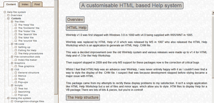
This package provides an alternative to the MS HTML Help Workshop and the WinHelp Workshop to allow you to create HTML Help files for VB packages where you have complete control of the styling of all aspects of the display.
Click here to download HTML Help, (174K).
Downloads
Map editing for HTML

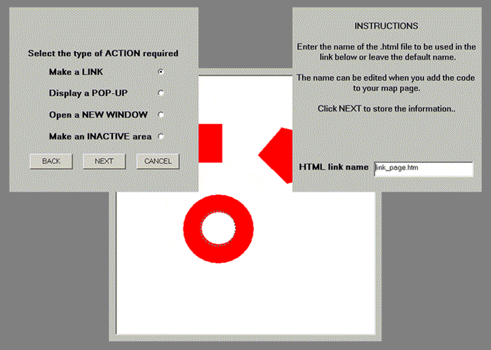
The MAP EDITOR package allows you to create "hot-spot" areas on images for .HTM files.
As well as defining the type and coordinates of the area, the program produces HTML code for the action required:
- A link,
- A Pop-Up,
- Opening a New Window or
- An inactive area.
Downloads
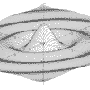
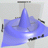
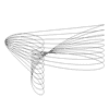
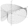
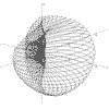
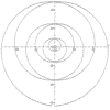
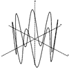
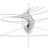
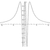
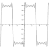
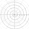
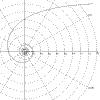
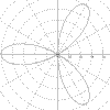
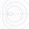
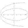
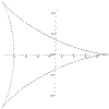
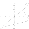
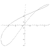
Function Graphing in 2 and 3D

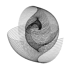
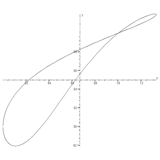
These are functions of the form:-
- z = f(x, y),
- x = f1(u,v), y = f2(u,v), z = f3(u,v)
- r = f(a, b),
- x = f1(t), y = f2(t), z = f3(t)
- r = f1(t), a = f2(t), z = f3(t)
- z = f(r, a),
- y = f(x),
- r = f(a) and
- x = f1(t), y = f2(t)
The functions can be plotted without or with axes which can be scaled and the resolution of the graph can be changed to facilitate speed of plotting.
Up to 10 different functions of the same type can be overlaid with each being drawn in a different colour.
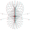
The 3D functions can be displayed and printed in one of two stereo forms: stereo-pairs or red/blue anaglyphs.
Functions can be stored and any number of different storage files created. There is also an extensive "Help" file included.
The package now allows 3D surface plotting with some forms of graph, courtesy of the Surface Viewer control by Bright Ideas Software
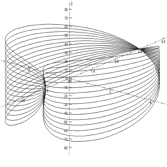
Other graphing sites:-
Downloads
Graph Gallery, page 1

Click a thumb-nail graphic for an enlarged version.
Downloads
Graph Gallery, page 2

Click the thumb-nail graphic for an enlarged version.
Downloads
Dawkins' Biomorphs

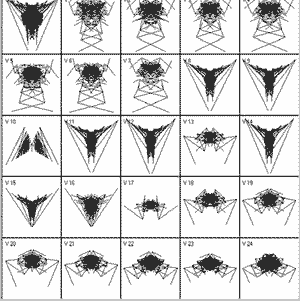
This version lets you display a particular biomorph and all its relations produced by a change of 1 in each gene value or a set of 25 random mutations from a particular biomorph, as shown on the left.
Each type of display can be printed, either as a grid display or as a full-size biomorph, and they can be saved in storage files of which any number can be created.
A sample storage file is included in the package and there is also an extensive "Help" file appended.
Click here to download BIOMORPHS, (2.28M).
Other Biomorph sites:-
Downloads
MANDELBRÖT & JULIA SETS


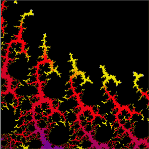
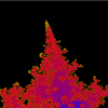
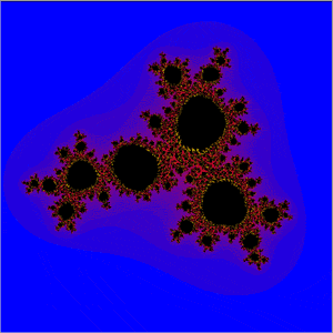
This version allows you to draw the Mandelbröt sets for ten different iterative functions and their associated Julia sets.
| Function | Real part | Imaginary part |
| z = z² + c | x² - y² | 2xy |
| z = z³ + c | x³ - 3xy² | 3x²y - y³ |
| z = z² + z + c | x² - y² + x | y(2x + 1) |
| z = z² - z + c | x² - y² - x | y(2x - 1) |
| z = z(z² - 1) + c | x³ - 3xy² - x | 3x²y - y - y³ |
| z = z²(z - 1) + c | x³ - x² - 3xy² + y² | 3x²y - 2xy - y³ |
| z = z² - z - 1 + c | x² - y² - x - 1 | y(2x - 1) |
| z = z⁴ + c | x⁴ - 6x²y² + y⁴ | 4(x³y - xy³) |
| z = z(z + i) + c | x² - y² - y | x(2y + 1) |
| z = z²(z + i) + c | x³ - 3xy² - 2xy | 3x²y + x² - y² - y³ |
Areas for enlargement are selected by dragging the mouse over a display and displays can be printed and stored, either as the basic data used to generate the display or as the actual display data.
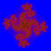
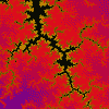
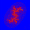
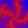
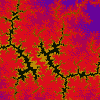
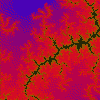
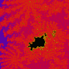
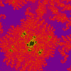
The illustrations are areas of the sets produced by the function z = z²(z - 1) + c
A sample storage file is included in the package and there is also an extensive "Help" file appended.
The current version has had a number of modifications added, the most important of which is that you can now enter your own equations.

Other Mandelbröt sites:-
- Julia and Mandelbröt Sets
- Images of the Filled Julia Set for the Riemann Zeta Function
- Fractal Explorer Mandelbröt and Julia sets (by Fabio Cesari)
- Julia Set, Mu-Ency at MROB
- Mandelbröt Set and Julia Sets
- Mandelbröt And Julia Set Explorer
- Julia and Mandelbröt Set Bibliography
- The Fractory Make-Your-Own Julia Sets
- Mandel and Julia
- Mandelbröt and Julia sets
Downloads
The MANDELBRÖT & JULIA GALLERY, page 1

(the coordinates of the lower-left corner, followed by the length of the side). The constant is added for Julia sets.
Most values are shown in exponential notation.
Click the thumb-nail graphic for an enlarged version.
Downloads
The MANDELBRÖT & JULIA GALLERY, page 2

(the coordinates of the lower-left corner, followed by the length of the side). The constant is added for Julia sets.
Most values are shown in exponential notation.
Click the thumb-nail graphic for an enlarged version.
Downloads
STATS, an interactive statistics package

The package allows investigation of a range of statistical operations by the use of an interactive, command driven system.
Data can be entered from the keyboard, generated by commands or imported from Excel workbooks or Access databases.
A simple interpreted language is included to allow the programming of commands.
Data can be stored and re-loaded as can sets of commands or programs.
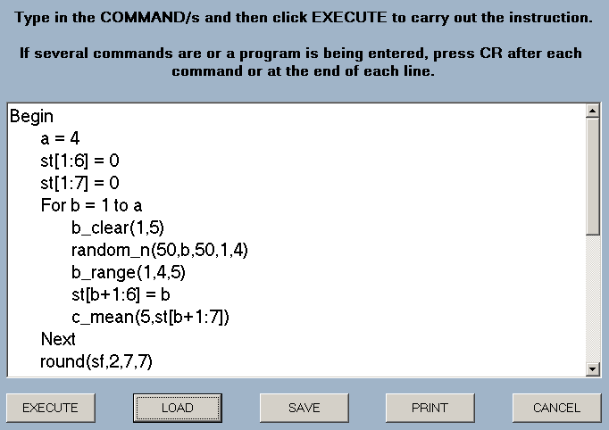
The package includes an extensive Help file which illustrates the various operations and gives sample programs including that shown in the Command window on the right.
or download the STATS package, (5.2M).
Downloads
STATS commands index

The command syntax requires that NO SPACES are used within a command. A list of abbreviated commands can be added to the display by right-clicking the text above the command window.
Where there are commands whose only difference is that one operates on a block of data whilst the other processes a column, the command is prefaced by 'b' or 'c' to indicate which is which.
e.g.'b_range' finds the ranges across the rows of a block of data whilst 'c_range' finds the range of the data within the specified column.
The commands are shown with the command in bold and the required parameters in italics. This is followed by a description of the command and an illustrative example.
Some commands require a variable name as a parameter to return the result of an operation.
Descriptions and examples of the commands can be found by clicking on the 'Commands' links in the following list.
| Commands 1 | CLEARING DATA | |
| clear_all | Clears all of the data. | |
| b_clear | Clears a block of data. | |
| DATA STORAGE | ||
| save_data | Saves a block of data. | |
| load_data | Load a stored block of data or data from Access or Excel files. | |
| DATA PRODUCTION | ||
| enter_data | Enter data from the keyboard. | |
| seq | Generate a sequence of values. | |
| fib | Generate a Fibonacci like sequence of values. | |
| function | Generate pairs of values from a specified function. | |
| concat | Concatenate two columns of data. | |
| random_i | Generate a set of random integers. | |
| random_r | Generate a set of random real numbers. | |
| random_n | Generate a set of random reals with a specified Standard Deviation and mean. | |
| random_be | Generate a set of random ones and zeroes with a Bernoulli distribution. | |
| random_bi | Generates a set of random integers with a Binomial distribution. | |
| random_p | Generate a set of random integers with a Poisson's distribution. | |
| random_x | Generate a set of random integers with an exponential distribution. | |
| Commands 2 | DATA OUTPUT | |
| display | Displays a block of data. | |
| value | Displays the current value of a program variable. | |
| histogram | Displays histogram or other bar chart. | |
| point_plot | Displays scattergrams of data. | |
| graph | Displays graphs of data. | |
| best_line | Draws the best line through a set of data. | |
| find_line | Draws a set of 'best-fit' lines through a set of data. | |
| Commands 3 | ARITHMETIC OPERATIONS | |
| b_sum | Adds the values in the rows of a block of data. | |
| c_sum | Adds the values in a column of data. | |
| diff | Subtracts one column from another. | |
| inc | Adds a constant to the values in a column of data. | |
| scale | Multiplies a column by a constant. | |
| b_min_max | Finds the maximum and minimum values in a block of data. | |
| c_min_max | Finds the maximum and minimum values in a column of data. | |
| b_range | Finds range of values across the rows of a block of data. | |
| c_range | Finds range of values in a column of data. | |
| b_mean | Finds the mean value of the rows in a block of data. | |
| c_mean | Finds the mean value of a column of data. | |
| parsum | Finds the partial sums of a column of data. | |
| sigma | Finds the sum of the products of two columns of data. | |
| replace | Replaces specified values in a column of data. | |
| s_d | Finds the Standard Deviation of a column of data. | |
| dist | Finds the distribution of the data of a column. | |
| sort | Sorts a column of data. | |
| regress | Allows regression values onto a 'best line' to be found. | |
| round | Rounds a column of data to a specified number of decimal places or significant figures. | |
| Commands 4 | SIGNIFICANCE TESTS | |
| correlate | Finds the product-moment correlation coefficient. | |
| chi_test | Carries out a χ² test. | |
| t_test | Carries out the 'Student's' T-test. | |
| m_w_test | Carries out a Mann-Whitney test. | |
The interpretation of the commands and the evaluation of expressions make use of the Microsoft document, Q86688, which has been expanded to deal with more user variables.
Downloads
STATS commands, page 1

CLEARING DATA
clear_all
Clears all data to zero.
b_clear(first column number, last column number)
Clears the block of columns to zero.
e.g. b_clear(3,6) will zero all values in columns 3 through to 6.
DATA STORAGE
save_data( first column number,second column number)
This saves the block of data defined by the two column numbers.
e.g. save_data(1,4) will save all the data in columns 1 to 4.
load_data(column number)
This loads a block of data, starting the storage at the specified column number. The data is added below any existing data in the columns concerned,
e.g. load_data(2) will load a block of data, starting the storage in column 2 and continuing for the number of columns in the block.
If STATS data is being re-loaded, a parameter of zero will re-load it into the same columns from which it was saved. Otherwise, it's loaded into the specified column onwards. A parameter of zero will give an error with Access or Excel data.
Executing the command first displays the data file selection screen.
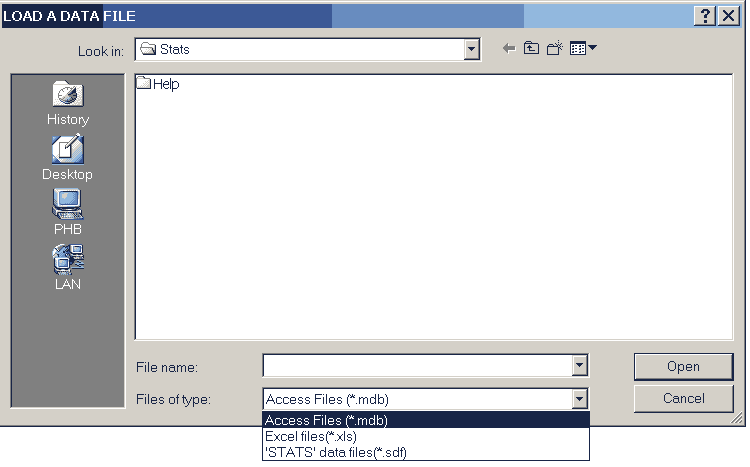
Three types of data file can be loaded.
- MS Access databases, (.MDB files),
- MS Excel workbooks, (.XLS files), and
- STATS custom datafiles, (.SDF files).
DATA PRODUCTION
enter_data(number of items, first column number, last column number)
Allows the specified number of items to be entered from the keyboard into a block of columns, a row at a time.
e.g. enter_data(50,1,3) will allow the entry of 50 rows of data into columns 1 to 3.
If data already exists in the block the entered data is added to the existing so, if this is not wanted, clear_all or b_clear should first be used to remove the existing data.
Clicking the CANCEL button will stop the process; saving the last complete row of data.
seq(initial value,geometric factor,arithmetic factor,number of items,column number)
This will produce a sequence of numbers in the specified column using the first three parameters in a recurence relationship of the form un+1 = g un + a where u1 is the initial value and g and a the geometric and arithmetic factors.
e.g. seq(1,2,1,7,4) will produce the sequence 1, 3, 7, 15, 31, . . . in column 4.
fib(initial value,second value,first term factor,second term factor,number of items,column number)
This will produce a sequence of numbers in the specified column using a recurence relationship of the form un+2 = a un + b un+1 where u1 is the initial value, u2 is the second value, a is the first term factor and b is the second term factor.
e.g. fib(1,2,1,1,20,1) will produce the Fibonacci sequence, 1, 2, 3, 5, 8, 13 . . ., for 20 terms in column 1.
function(function,start value,end value,step value ,x-data column number,function column number)
This will produce a sequence of numbers where the values in the column correspond to the X-data generated by the start value, the end value and the step value and the Function column contains the corresponding values of the function.
The function must be entered with 'x' as the variable using standard BASIC syntax.
e.g. function(x^2,1,8,2,1,3) will produce the values 1,3,5,7 in column 1 and the corresponding squares in column 3.
concat(column1,column2)
Extends the data in the first column by adding on the data from the second.
e.g. concat(3,5) will add the data in column 5 to that already in column 3.
The largest number of data creation commands are to produce sets of random numbers.
random_i(lower limit,upper limit,number,first column number, last column number)
This produces a set of random integers with a rectangular distribution between the specified limits in the designated block of columns.
e.g. random_i(1,6,50,3,5) will simulate 50 rolls of a die in columns 3 to 5.
random_r(lower limit,upper limit,number,first column number, last column number)
This produces a set of random real numbers with a rectangular distribution between the specified limits in the designated block of columns.
e.g. random_r(2.5,3.5,10,1,2) will generate 10 numbers in each of columns 1 and 2 with values between 2.5 and 3.5
random_n(mean,standard deviation,number,first column number,last column number)
This generates a set of normally distributed random real numbers with the specified standard deviation and mean in the designated block of columns.
e.g. random_n(20,2,50,3,5) will generate 50 numbers in columns 3 to 5 where the numbers in each column have a mean of 20 and a standard deviation of 2.
random_be(probability,number,first column number,last column number)
This generates a set of random ones and zeroes in the designated block of columns according to a Bernoulli distribution.
e.g. random_be(0.35,10,7,9) will produce a set of 10 0's and 1's in each of columns 7 to 9 where the probability of a 1 is 0.35.
random_bi(trials,probability,number,first column number,last column number)
This generates random integers with a Binomial distribution specified by the 'trials' and probability values in the designated columns.
e.g. random_bi(10,0.8,20,5,8) will produce 20 numbers in each of columns 5 to 8 where each value is the number of successes in 10 trials where the probability of a success was 0.8.
random_p(mean,number,first column number,last column number)
This generates random integers with a Poisson's distribution which represents the number of occurences with the specified mean within a unit interval.
e.g. random_p(10,100,1,2) will produce 100 random integers in each of columns 1 and 2 which have a mean value of 10 and a Poisson distribution.
random_x(mean,number,first column number,last column number)
This generates random integers with an exponential distribution which represents the number of intervals with the specified mean value between two events.
e.g. random_x(4,20,3,5) will produce 20 random integers with a mean of 4 in each of columns 3 to 5 with an exponential distribution.
Downloads
STATS commands, page 2

display(output device,first column number,last column number)
This will output the contents of the specified columns to either the screen or printer depending on the output device parameter, (screen or printer).
e.g. display(screen,1,6) will display the contents of columns 1 to 6 on the VDU.
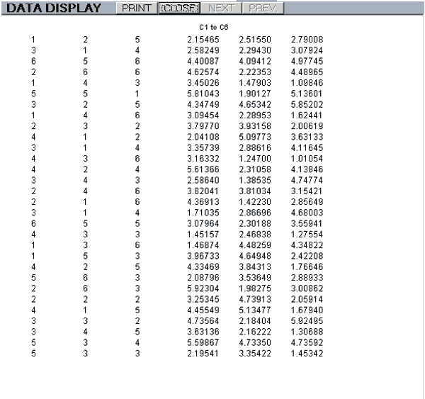
A screen display has buttons to select the NEXT and PREVious pages, when applicable, and a PRINT button.
If the data can be identified as integer it is displayed with no decimal points. Otherwise, it is rounded to 4 d.p. no matter how many places there are.
The maximum size of a display page is 53 rows of 7 columns.
value(object name)
This will display on the screen the current value of the object concerned which can be a program variable or an element of data using the st[row:column] notation.
e.g. value(pp[2]) will display the current value of the second element of the pp[ ] array.
histogram(dimensions,type,steps,first column number,last column number)
This will display on the screen histograms of the data in the selected columns.
The acceptable values for the first two parameters are:-
| Dimensions | |
| Values | Result |
| 2D | A two dimensional display |
| 3D | A three dimensional display |
| Type | |
| Values | Result |
| hist | Histogram |
| p_d_f | Probability density function |
| c_d_f | Cumulative distribution function |
e.g. histogram(2D,hist,6,1,3) will display a 2-dimensional histogram with three sets of bars representing the data in columns 1 to 3, split into 6 steps.
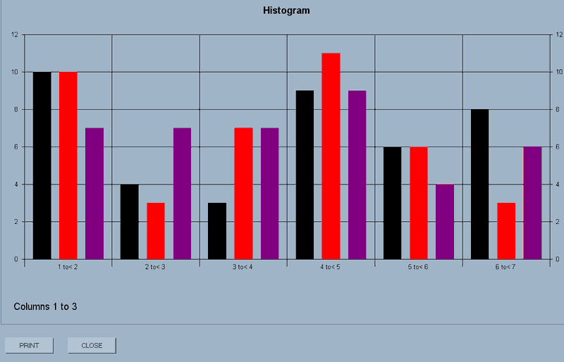
The display has a PRINT and CLOSE button.
N.B.3D displays can be rotated around their axes by holding down the CTRL key, left-clicking the mouse and dragging.
point_plot(axes,first column number,last column number)
This will display on the screen scattergrams of the data in the columns concerned.
e.g. point_plot(axes,1,3) will display scattergrams of the data in columns 1 to 3.
The 'axes' parameter, (axes or no_axes), defines whether axes are to be drawn for this plot.
Essentially, this allows you to overlay several sets of data by selecting 'axes' for an initial plot and then 'no_axes' for a subsequent plot or plots.
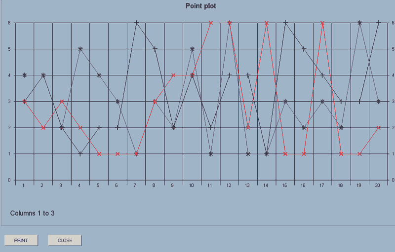
If you then use point_plot(no_axes,6,7), the plots for the data in columns 6 and 7 will be added to the display.
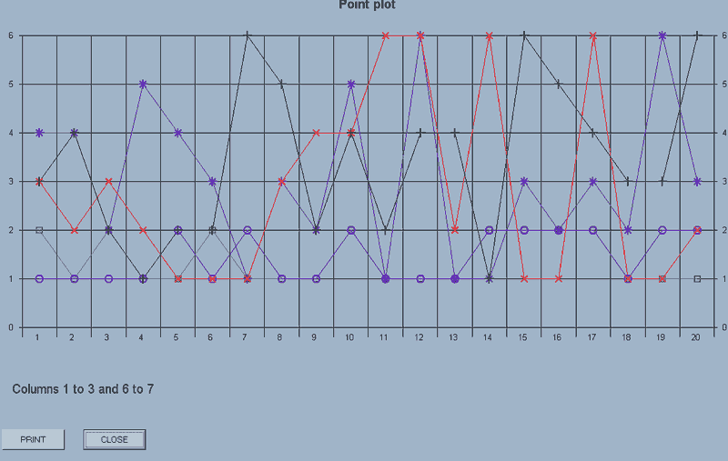
The display has a PRINT and CLOSE button.
Each set of data is plotted using a different symbol up to the maximum of 8 sets of data.

The maximum number of points which will be displayed is 30. If there are more than this in a selected column, a sample is taken rather than having an error message displayed.
If there are different number of points in a block of columns, it's the first column which is used to set the number for display.
graph(axes,markers,x-data column number,first y_data column number,last y_axis column number)
The data in the x-axis column is plotted against that of each of the columns in the block of y-axis data.
e.g. graph(axes,markers,1,2,4) will draw graphs with point markers, where the X-data is that in column 1 and there are three graphs corresponding to Y-data in columns 2 to 4.
The acceptable values for the first two parameters are:-
| Axes | |
| Values | Result |
| axes | Axes are added to a new graph |
| no_axes | Subsequent plots are added to an existing graph. |
| Markers | |
| Values | Result |
| markers | Points are emphasised with the same markers used for 'point_plot' |
| no_markers | No markers are used. |
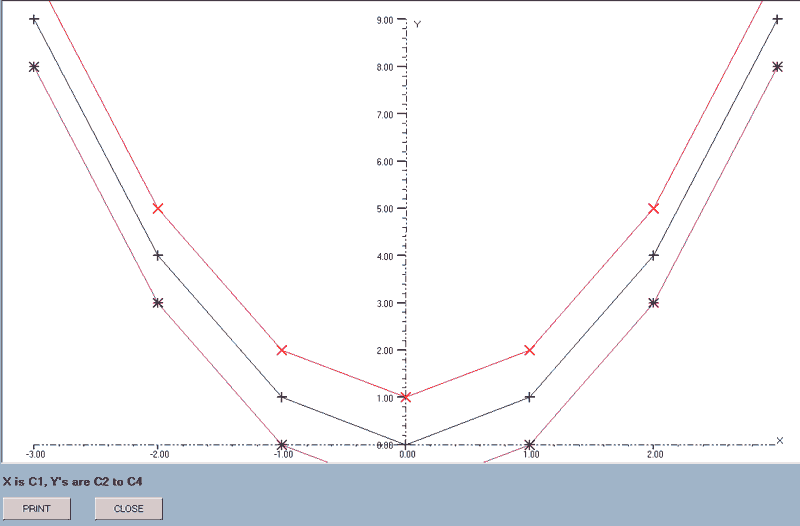
The axes ranges are calculated from the X-data column and the first of the Y-data columns. The actual range is rationalised to give ranges in simple numbers and the axes do not pass through the origin if this is not within the range of the data.
The X-data column can be included within the block but will be skipped as the graphs are drawn. e.g. graph(axes,markers,3,1,6) is acceptable: column 3 provides the X-data and graphs will be drawn using columns 1, 2, 4, 5 and 6 as the Y-data.
best_line(axes,type,x-data column number,first y_data column number,last y_data column number)
This will find the best line that fits the sets of data: the data in the x-axis column being plotted against that of the block of y-axis data.
e.g. best_line(axes,quad,1,2,4) will draw the best quadratics for the data sets where the X-data is that in column 1 and there are three graphs corresponding to Y-data in columns 2 to 4.
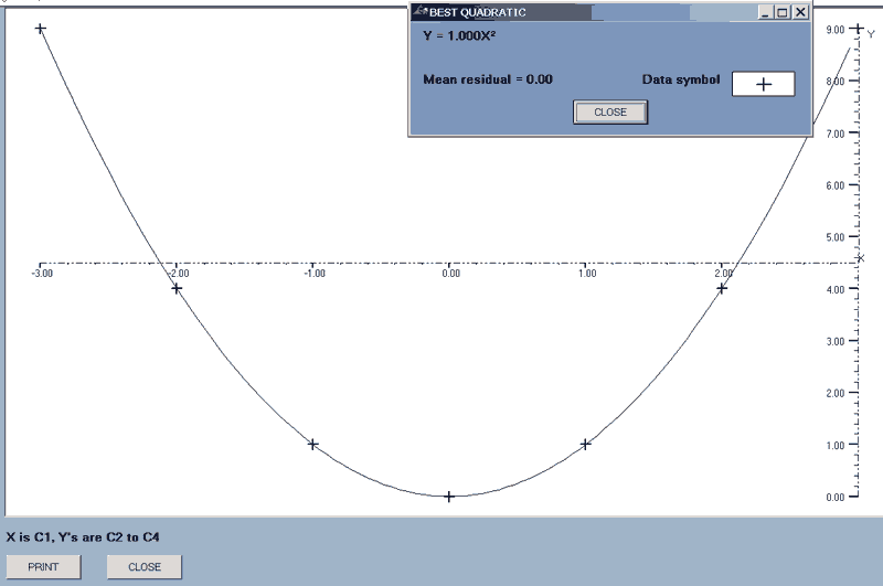
After each line is drawn, there is a display of the equation of the line concerned, the mean relative residual, (MRR), and the symbol used for the data points.
Each residual = data - function value and the MRR is defined as
Σ(absolute residuals)/Σ(absolute data).
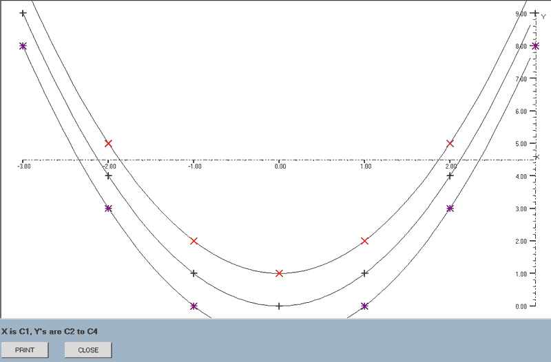
The acceptable values for the first two parameters are:-
| Axes | |
| Values | Result |
| axes | Axes are added to a new graph |
| no_axes | Subsequent plots are added to an existing graph. |
| Type | |
| Values | Result |
| linear | The best straight line is found. |
| quad | The best quadratic is found. |
| ab^x | The best line of the form y = a(bx) is found. |
| ax^r | The best line of the form y = a(xr) is found. |
The X-data column can be included within the block but will be skipped as the graphs are drawn. e.g. best_line(axes,linear,2,1,4) is acceptable: column 2 provides the X-data and graphs will be drawn using columns 1, 3 and 4 as the Y-data.
find_line(x-data column number,y_data column number)
This plots all of the available lines of best-fit for the data in the specified columns.
The mean relative residual for each line is stored and, if the graphs are printed, this information is added to the display as described above for the 'best_line' command and the minimum M.R.R. is listed as an aid in deciding which is the best line for this data.
A check is made at the start to see if the X or Y ranges include zeroes and, if they do, the two power graphs, y = a(bx) and y = a(xr), are excluded.
The first marker,
 , is used for the data and each line is drawn in a different colour.
e.g. find_line(1,2) will draw the four lines for the data in columns 1 and 2.
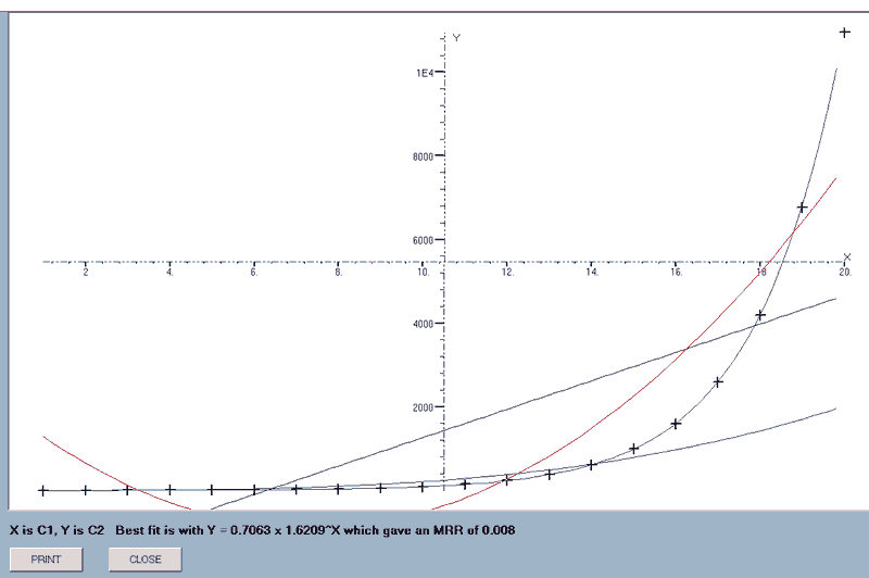
When all the graphs have been drawn, the equation of the one giving the smallest MRR is appended to the data display which, in this case, is the Fibonacci series!
Downloads
STATS commands, page 2: Arithmetic operations

b_sum(first column number,last column number,results column number))
This adds the values across a row and stores the result in the 'results' column.
e.g. b_sum(1,3,4) will add the values in each row of columns 1 to 3 and store the result in the corresponding row of column 4.
c_sum(column number,label)
This adds the values in the designated column and stores the answer with the specified variable name.
e.g. c_sum(5,c) will add the values in column 5 and store the result with the program variable name, c.
diff(first column number,second column number,results column number)
This subtracts the values in the second column form those in the first and stores the results in the results column.
e.g. diff(6,3,7) will subtract the values in column 3 from those in column 6 and store the results in column 7.
inc(amount,column number,results column number)
This will add the amount to each item in the specified column and store the result in the results column.
e.g. inc(-1.25,1,2) will subtract 1.25 from each item in column 1 and store the results in column 2.
scale(amount,column number,results column number)
This will multiply each item in the specified column by the amount and store the results in the results column.
e.g. scale(0.87,3,5)) will multiply each item in column 3 by 0.87 and store the results in column 5.
b_min_max(first column number,second column number,minimum column number,maximum column number)
This finds the maximum and minimum values in the specified block of data and stored the results in the minimum and maximum columns.
e.g. b_min_max(1,4,5,6) will find the minimum and maximum values in each row of columns 1 to 4; storing the minima in column 5 and the maxima in column 6.
c_min_max(the column number,variable for minimum,variable for maximum)
This finds the maximum and minimum values in the designated column and stored the results in the specified variables.
e.g. c_min_max(3,pp[0],pp[1]) will find the minimum and maximum values in column 3 and store the results in the array values pp[0] and pp[1].
b_range(the first column number,the last column number,the results column)
This finds the range of values across each row of the designated block and stores the value in the results column.
e.g.
b_range(3,5,6) will find the range of values across a row from column 3 to column 5 and store the result in column 6.
c_range(the column number,the result variable)
This finds the range of values within the designated column and stores the result with the specified variable name.
e.g. c_range(4,b) will find the range of values in column 4 and store the result as b.
b_mean(the first column number,the last column number,the results column)
This finds the mean of the values across each row of the designated block and stores the value in the results column.
e.g. b_mean(1,4,5) will find the mean of the values across a row from column 1 to column 4 and store the result in column 5.
c_mean(the column number,the variable for the result)
This finds the mean of the values in the designated column and stores the result with the specified variable name.
e.g.
c_mean(7,d) will find the mean of the values in column 7 and store the answer as variable d.
parsum(the first column number,the second column number)
This finds the partial sums, (cumulative totals), of the data in the first column and stores the results in the second column.
e.g.
parsum(4,6) will find the partial sums of the data in column 4 and store them in column 6.
sigma(the first column number,the second column number,label)
This finds the sum of the products of the values in the specified columns and stores the result with the designated variable name.
e.g. sigma(1,5,d) will multiply each element in column 1 by the corresponding item in column 5 and store the total of the products with the label d.
replace(lower limit,upper limit,replacement,the column number,the results column number)
This checks the data in the first column and, if the value, v, is such that lower limit ≤ v ≤ upper limit, v is replaced by the replacement value in the results column. Otherwise, the original value is transferred to the results column.
e.g. replace(1.1,2.3,0,1,2) will transfer the data from column 1 to column2, replacing the value by zero if 1.1 ≤ value ≤ 2.3
s_d(the column number,label for the result)
This finds the Standard Deviation of the data in the designated column and stored the value with the specified variable name.
e.g. s_d(5,x) will find the Standard Deviation of the data in column 5 and store it as variable x.
N.B. This will produce a result for any set of data but will only have validity if the data is normally distributed.
dist(type,interval,the column number,the results column number,label for the initial value, (the minimum))
e.g. dist(c_d_f,10,4,5,d) will find the cumulative distribution of the data in column 4 over 10 steps and store the results in column 5 with the minimum value being stored as variable d.
This was developed as part of the 'histogram' command but may have some use in its own right.
The 'type' parameter takes the same values as in 'histogram'. The command will find the distribution of the data in the designated column and stores the results in the results column with the initial, (minimum), value stored with the specified label.
sort(the number of fields,the order,the first column number,the last column number,the first results column number,the key column numbers)
The command allows a block of data to be sorted on any number of key columns which can be used in any order.
e.g. sort(3,ascend,1,4,5,1,2,4) will sort the data in the block of columns 1 to 4 in ascending order using as the 3 key fields column 1, then column 2 and finally column 4. The sorted data is stored in a block starting at column 5.
The 'order' parameter takes the values ascend or descend.
If the sorted data is to replace the original set, then the results column number is made the same as the intial.
e.g. sort(3,ascend,1,4,1,1,2,4) for the example shown above.
regress(type,the X-data column number,the Y-data column number)
A form is displayed which allows the entry of X-values and displays the corresponding Y-value on the basis of regression onto the designated line.

e.g. regress(quad,1,2) will find the quadratic of best fit to the data in columns 1 and 2 and display a form for the entry of X-values.
The 'type' parameter takes the same values as in 'best_line'.
round(type,number of figures,the source column number,the results column number)
The items in the source column are rounded according to the specification and stored in the results column.
The 'type' parameter takes the values 'dp' or 'sf'.
| Type | |
| Values | Result |
| dp | Rounding to decimal places |
| sf | rounding to significant figures |
e.g. round(sf,3,1,2) will round the data in column 1 to 3 significant figures; storing the results in column 2.
Dowloads
STATS commands, page 2: Significance tests

Several significance tests can be carried out using the basic commands, e.g. those involving means, so those included as specific commands are the ones which would be difficult to do via a series of arithmetic commands.
Probability and distribution tables will have to be used as it isn't thought to be efficient to tie up your PC's memory with pages of tables.
The tests will give results for any set of data but they will only have significance if the data is of a nature to which the test can be applied.
correlate(first column number,last column number,label))
This finds the product-moment correlation coefficient between the data in the designated columns and stores the result with the specified variable name.
e.g. correlate(3,4,x) will find the product-moment correlation coefficient between the data in columns 3 and 4 and store it as variable x.
chi_test(observed frequency column number,expected frequency column number,label))
This carries out a χ² test on the data in the first column by comparison with that in the second. The statistic, χ², is stored with the specified variable name.
e.g. chi_test(1,2,x) will compare the data in column 1 with the expected frequency of this data in column 2 and store the coefficient as variable x.
t_test(column number,quoted mean,label))
This carries out the 'Student's' T-test on the data in the column, which is compared with the quoted mean. The result is stored with the specified variable name.
e.g. t_test(1,2.3,c) will compare the data in column 1 which may be part of a set which has a mean value of 2.3; storing the result as variable c.
m_w_test(tails,end,first column number,second column number,label))
This carries out a Mann-Whitney test on the data where the acceptable values for 'tails' and 'end' are shown below.
| Tails | |
| Values | Result |
| one | Applies a one-tailed test. |
| two | Applies a two-tailed test. |
| End | |
| Values | Result |
| high | The high end of the distribution is used. |
| low | The low end of the distribution is used. |
e.g. m_w_test(one,high,1,2,a) will carry out a single-tailed test on the high end of the distribution of the data in columns 1 and 2; storing the result as the variable a.
Even though the 'end' parameter has no meaning in a two-tailed test, a value must be entered to avoid a syntax error. In fact, the algorithm assumes a symmetrical distribution, carries out the single-tailed test selected and multiplies the result by 2!
Downloads
Programing STATS commands

There is a limited set of programing commands which can be used to automate the use of STATS commands.
PROGRAM STATEMENTS
Whereas there must be NO spaces in STATS commands, programing statements MUST be spaced out except when using STATS commands or expressions.
Square brackets, [ ], indicate optional syntax.
The start an end of a set of instructions must be stated explicitly.
Begin must be at the start of a program.
Finish must be at the end of a program.
The application has a number of in-built numeric variables which can be used to store the results of operations or in programs.
These are:-
| a, b, c, d, l, m, x, y | Simple numeric variables. |
| pp[ ] | An array variable which can have subscript values from zero, (pp[0]), up to the current number of columns, (pp[number of columns]). |
| st[row:column] | This is not strictly a variable but acts as one for the purposes of storing data and displays. It references an element of the stored data by row and column. e.g. st[3:2] refers to the third number in column 2. |
In the last two cases it is essential to use square brackets, [ ], rather than round ones.
The program also allows you to use pi, (p), and e
ASSIGNMENT= assigns a variable name to value.
The value may be an actual number, another variable or an expression created using standard BASIC syntax.
e.g. b = 2*c-d will assign the current value of the expression 2*c-d to the variable b
For variable name= starting value to final value [step step value]
This statement defines the start of a loop where the loop variable takes the specified values.
'Step' values can be fractional and negative. If no 'step' is included, it defaults to 1.
Loops may be nested.
e.g. For m = 1 to 5; will start a loop using m as the loop variable with initial value 1 which will increase by 1 each loop until a final value of 5 is exceeded.
Next
This defines the end of a loop. When this position is reached, the loop variable is incremented by the 'step' value and checked against the final value defined in this loop's 'For' statement. If the end of the loop has been reached, the loop is terminated. Otherwise, the program loops back to the line after the 'For' statement.
Do ... While or Do ... Until loops can be faked by a For ... Next loop, although, with hindsight, it might have been easier to define a Do loop and fake a For ... Next!
If condition then
This statement checks the truth of the specified condition.
If it is True then the lines following the statement are processed until an 'Else' or 'Endif' statement is found. Otherwise, the lines following the corresponding 'Else' or 'Endif' statements are processed.
If a>= 7 then; will continue with the next lines if the value labeled a is currently greater than or equal to 7.
[Else]
If an 'Else' statement is included, it is the lines following this which will be processed when the 'If' condition is False
Endif
If there is no 'Else' statement, the program jumps to the lines after 'Endif' when the 'If' condition is False.
' The single quote symbol allows you to add explanatory comments to your programs.
These can come at the end of a progam line e.g. For a = 1 to 7 'Loop seven times.
or have a line to themselves. e.g. 'The next section generates random integers.
The following senior school investigation is used as an example to illustrate the use of repetition.
"Investigate the range produced and the mean of the range when a set of normally distributed random numbers are generated with different Standard Deviations."
Using STATS commands alone, the following will produce the required information.
random_n(50,1,50,1,4)
b_range(1,4,5)
c_mean(5,a)
value(a)
The process would then need to be repeated with the Standard Deviation in the 'random_n' command changed to 2, then 3, etc.
This calls for a program and a loop! (With comments added for clarity).
| Begin | |
| For a = 1 to 4 | 'Use a For loop to generate Standard Deviations. |
| clear_all | 'Clear out the previous set of data. |
| random_n(50,a,50,1,4) | 'Generate 50 random numbers with a mean of 50 and S.D. a in columns 1 to 4. |
| b_range(1,4,5) | 'Find the range if the values in columns 1 to 4 and store the result in column 5. |
| c_mean(5,b) | 'Find the mean of the ranges and store the result as b. |
| value(b) | 'Display the mean |
| Next | |
| Finish |
This will provide the required information but it can be made better by having it store the results and draw a best line through them.
| Begin | |
| a = 4 | 'Use a variable to define the number of loops. |
| st[1:6] = 0 | 'Store a zero in the first row of column 6 |
| st[1:7] = 0 | 'and column 7 as the first data pair. |
| For b = 1 to a | 'Use a For loop to generate Standard Deviations of 1 to a. |
| b_clear(1,5) | 'Clear the working block of data, columns 6 & 7 must stay. |
| random_n(50,b,50,1,4) | 'Generate 50 random numbers with a mean of 50 and S.D. b in columns 1 to 4. |
| b_range(1,4,5) | 'Find the range if the values in columns 1 to 4 and store the result in column 5. |
| st[b+1:6] = b | 'Store the Standard Deviation in column 6 |
| c_mean(5,st[b+1:7]) | 'and the mean of the ranges in column 7 |
| Next | |
| best_line(axes,linear,6,7,7) | 'Show the best straight line for the means plotted against the Standard Deviations. |
| Finish |
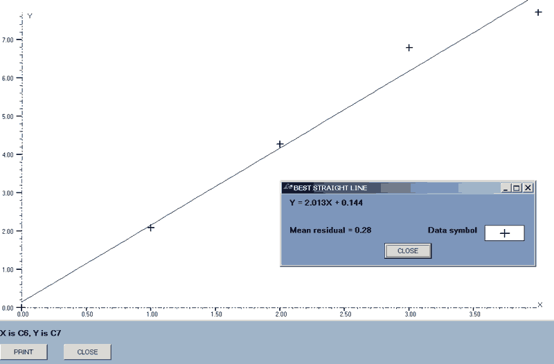
I feel that the use of conditional statements is likely to be limited in the context of STATS.
The following example is given as a simple illustration of 'If ... then', 'Else' and 'Endif' for anyone not familiar with the structure.
| Begin | |
| For a = 1 to 5 | 'Use a For loop. |
| If a>2 then | 'Start of the conditional statement. |
| b = 3 | 'Assign b the value 3 if the condition is True, |
| Else | 'Otherwise, |
| b = 2 | 'assign it the value 2. |
| Endif | 'The end of the conditional statement. |
| value(b) | 'Display the value of b, (2, 2, 3, 3, 3) |
| Next | |
| Finish |
It is possible to indent program statements to emphasise the structure by the use of spaces, (Tabs won't work), and the F10 key is programmed to add or insert a group of spaces into a line which has no effect on the execution of a program.
| Begin |
| For a = 1 to 5 |
| If a>2 then |
| b = 3 |
| Else |
| b = 2 |
| Endif |
| value(b) |
| Next |
| Finish |
It would be simple to extend the program facility to allow the use of any variable name; of different variable types and of extra programing statements. As mentioned previously, this has not been done because it would carry an overhead of processing time which will slow down the interpreter.
However, if you feel that extra facilities would be useful, please contact me.
Downloads
BASIC syntax

It may be that my references to 'BASIC syntax' might not mean much to some people.
It used to be that every small computer came equipped with BASIC but, as this has not been the case for some years now, I felt it might be useful to give a brief outline of the BASIC syntax you need to use to enter equations for the 'function' command or to create expressions for a program or command.
BASIC is an acronym for Beginners All-purpose Symbolic Instruction Code and it is the language that most of us over cut our programming teeth on. Over and you were likely to have started programming in binary via a set of switches!
The operators and functions which you can use are listed below. They are all case sensitive.
OPERATORS
Recognised operators in order of precedence.| Package code | Operation |
| ^ | Raise to the power |
| * | Multiplication |
| / | Fractional, floating point division |
| \ | Integral division |
| mod | Mod, Modulus |
| + | Addition or a positive value |
| - | Subtraction or a negative value |
| = | Equality |
| > | Greater than * |
| Less than * | |
| <> | Not equal to * |
| <= | Less than or equal to * |
| >= | Greater than or equal to * |
| and | Logical AND * † |
| or | Logical OR * † |
| xor | Logical Exclusive OR, XOR * † |
| not | Logical NOT * † ‡ |
| eqv | Logical equivalence, Not XOR * † ‡ |
| imp | Logical implication * † ‡ |
* The results of logical operations return -1 for True and 0 for False.
†
These operators can be applied to values as well as conditions.
Hover over the reference symbols for examples.
‡ These operators can generate 1's from zeroes. As all of the bits in the number/s are processed, (32 bits in the case of integers), any leading zeroes in the values used will generate 1's and so the result is likely to be a negative number.
Hover over the symbols for examples.
FUNCTIONS
| Standard Functions | |
|---|---|
| Package code | Function |
| abs | Abs, the absolute value |
| cos | Cos, cosine |
| exp | Exp, enumber, the antilogarithm |
| fix | Fix, = Sgn(number)*Int(Abs(number)) |
| int | Int, the integer portion of the number |
| log | Log, the natural logarithm |
| rnd | Rnd, a random number where 0 ≤ number < 1 |
| sgn | Sgn, sign of the number |
| sin | Sin, sine |
| sqr | Sqr, the positive square root |
| tan | Tan, tangent |
| Derived Functions | |
| Package code | Function |
| log10 | Logarithm to the base 10 |
| log2 | Logarithm to the base 2 |
| Inverse Trig. Functions | |
| Package code | Function |
| sec | 1/Sin, secant |
| cosec | 1/Cos, cosecant |
| cot | 1/Tan, cotangent, cotan |
| arcsin | 'Angle whose sine is' |
| arccos | 'Angle whose cosine is' |
| atn | 'Angle whose tangent is', Arctan |
| arcsec | 'Angle whose secant is' |
| arccosec | 'Angle whose cosecant is' |
| arccot | 'Angle whose cotangent is' |
| Hyperbolic functions | |
| Package code | Function |
| sinh | Hyperbolic Sine |
| cosh | etc. |
| tanh | |
| sech | |
| cosech | |
| cotanh | |
| arcsinh | |
| arccosh | |
| arctanh | |
| arcsech | |
| arcosech | |
| arccotanh |
With BASIC, the main rule is that everything has to be stated explicitly. e.g. we all know that 2x means "Two multiplied by x" but this has to be written in full as '2*x' in BASIC.
A second point is that, as all parts of an equation have to be entered in line, far more parentheses are needed than is the case with written algebra. An equation which would usually be written as "1 over 1 + x" has to be entered as 1/(1+x).
Whilst the following is a rule of basic arithmetic not BASIC, a common mistake is to misinterpret expressions such as 2 + 5 x 3 and expect the result '21' when, in fact, it's 17. [21 = (2 + 5) x 3].
Downloads
The EXCEL classes

Whilst being OK for the occasional macro, VBA has its limits for full projects. The syntax is more limited than that of VB and I've found stability problems with Excel VBA. However, Excel is a very useful data storage medium and the Excel classes were designed to allow this use from within a VB based application. However, I'm in the process of replacing Excel with LibreOffice Calc, (see the LibreOffice VB6 section), and may re-write these classes to work with LO.
There are two classes, ExcelApplication and ExcelWorkbook.
ExcelApplicationThis opens Excel if necessary and creates a collection for ExcelWorkbook objects. Ony one ExcelApplication object can exist at a time.
ExcelWorkbookThis allows workbooks to be opened and manipulated. Books are defined as 'With Events' so that use can be made of Excel events.
The class has the following methods and properties.
METHODS| Name | Parameters | Operation |
| open_book | Book name | Opens the specified book. |
| clear_sheet | Clears the contents of the current sheet. | |
| save_book | Saves the open book. | |
| close_book | Closes the open book. |
| Name | Parameters | Operation |
| get_book | Returns a reference to the open book object. | |
| sheet_name | Returns the name of the active sheet. | |
| get_sheet | Returns a reference to the active sheet. | |
| select_sheet | Sheet name | Selects the sheet and returns a reference to it. |
| set_sheet | Sheet name | Returns a reference to the specified sheet object WITHOUT selecting it. |
| set_range | Sheet name, (r1, c1), (r2, c2) | Returns a reference to the defined range on the specified sheet WITHOUT selecting it. |
The class contains a procedure for only one event, 'xlBk_SheetActivate', which calls a main program procedure, 'select_sheet_action', whenever a new sheet is selected. However, it is easy to add code for other events using these as templates.
Downloads
The PRINTING classes

These classes are designed to allow the layout, preview and printing of text from within a VB application.
There are two classes,
PPpages, which is used to create a set of pages and deals with operations which apply to the WHOLE SET, and
PPpage, which deals with the methods and properties applicable to a SINGLE page.
PPpages
This class has the following Methods and Properties,
| Method | Operation |
| Add | Add a page to a collection |
| delete | Delete a page from a collection |
| mt | Empty a collection |
| page_parms | Set the page parameters |
| set_pinc | Set the page number increment, 1 or 2 |
| change_v_bar | Change the vertical Scroll bar position † |
| change_h_bar | Change the horizontal Scroll bar position † |
| zoom | Zoom in or out, (Left click), to a maximum of 300% † |
| switch_zoom | Toggle the direction of zoom, (Right click). † |
| close_preview | Close the Preview form † |
| print_it | Print or preview the current page |
| select_printer | Select a printer † |
| select_Excel_printer | Select a printer for use with Excel workbooks |
| page_setup | Set page data via the 'Page Setup' window |
| font_setup | Set font data via the 'Font Setup' window |
| Property | Data |
| page_data | Return page data, margins, etc. |
| find_index | Return the collection index of a page |
| find_page | Return a 'page' object |
| font_dta | Return the current font data |
| page_col | Return a 'pages' collection object |
† These methods exist to be accessed by the Preview Form and should not otherwise be used.
The units used for page sizes can be set to either inches or mm. by means of a flag variable.
PPpage
This class has the following Methods and Properties,
| Method | Operation |
| set_object | Select an alternative to the Preview form for display |
| set_p_col | Set the background colour of the display object. |
| add_text | Basic text routine. * |
| add_f_text | More advanced text routine. * |
| add_graphic | Adds a graphic images to a page. * |
| terminate | Terminate a line of text. |
| set_sizes | Set the page data, margins, etc. † |
| set_align | Set a global alignment for a page. |
| page_numbers | Add the numbers of a page |
| set_zoom | Set the zoom factor |
| font | Set ALL font parameters |
| set_font | Set a SINGLE font parameter |
| set_pp | Set the Print/Preview flag |
| head_foot | Add header or footer text. * |
| super_date | Construct a date string with days shown as, e.g. 15th. |
† This method exists only to transfer page data from a PPpages object and should not otherwise be used.
| Property | Data |
| page_number | Return the Local or Absolute number of a page |
| page_flag | Return the current Print/Preview flag |
| page_data | Return page data, margins, etc. |
| font_defaults | Return ALL the font parameters from the PPpages object |
| font_data | Return a SINGLE font parameter |
| centre | Return an offset to centre a piece of text |
| line_height | Return the current line separation |
add_text is a basic text display routine. It will add a line of text formatted Left, Right or Centre but the text is truncated if longer than a line width.
add_f_text is a more versitile text display routine which will wrap excess text onto a new line, allow Full justification as well as Left, Right and Centre and will recognise the following, in-line font formating codes,
| Code | Action |
| \ | Start of formating code |
| / | End of formating code |
| b | Set font Bold |
| i | Set font Italic |
| u | Underline text |
| t | Strike through the text |
| s | Set as superscript |
| p | Set as subscript |
| k | Backspace |
| y | Select 'Symbol' font |
| w | Select 'WingDings' font |
| d | Reselect the default font |
| q[digits] | Set the corresponding QB colour |
| [digits] | Set the point size to the value |
| n | Return to default font values |
* More detail on the operation of these methods is given here.
Downloads
The PRINTING classes: TEXT and GRAPHIC methods

Basic addition of text
add_text(tx, hp, tm, ByRef p_d, Optional vp, Optional alg)
| Parameters | |
| tx | the TEXT, |
| hp | the HORIZONTAL position in units, which is updated and returned via the parameter, |
| tm | the LINE TERMINATOR flag, |
| p_d | the PRINT DEPTH in units, which is updated and returned via the parameter, |
| alg | the ALIGNMENT, 0 = Left, 1 = Centre, 2 = Right, defaults to -1 which accepts the current page alignment, |
| vp | the VERTICAL offset in units, defaults to zero, |
If the text is longer than the available page width as defined by the vertical margins and any horizontal offset set by 'hp', an error message is displayed but as much of the line will be printed as will fit on the page.
The line terminator flag is a Boolean which will terminate the text line if True. Setting it False allows further text to be added to the same line.
The alignment setting is really of little use! If you're going to add extra text on the same line, i.e. the termination flag is clear, only Left alignment can be allowed as is the case if there is already some text on the line, i.e. 'a non-zero 'hp'.
The vertical parameter, 'vp', which is set to default to zero, is an addition to the current printing depth, 'p_d', which can be used to add line spacing.
All text formating has to be carried out using the 'font' or 'set_font' methods.
Addition of formated textadd_f_text(tx, Optional p_d = 0, Optional tm As Boolean = False, Optional alg = -1, Optional p_l As Single = 0,
Optional vp As Single = 0, Optional h_p As Single = 0)
| Parameters | |
| tx | the TEXT, |
| p_d | the PRINT DEPTH in units, defaults to zero |
| tm | the LINE TERMINATOR flag, defaults to False |
| alg | the ALIGNMENT, 0 = Left, 1 = Centre, 2 = Right, 3 = Fully Justified, defaults to -1, (accept the current global alignment). |
| p_l | the PART LINE length in units, optional, default = zero, |
| vp | the VERTICAL offset in units, defaults to zero |
| h_p | the HORIZONTAL offset in units, defaults to zero |
If the printing depth is defaulted, the current internal value will be used. If a non-zero value is entered for the parameter, the internal value is reset to this figure.
The line terminator flag is a Boolean which will terminate the line at the end of the text block if True. The default of False allows further text to be added to the same line, (See PART LINE, below).
The alignment, 'alg', defaults to -1 which means that the current page alignment is used. This is either the default of Left or that set by the 'set_align' method.
The PART LINE value is used to return the position of the text on the line at the end of a block which can then be used to complete this line with further text, provided that the termination flag was set to False. N.B. If full justification is used, the first part of such a line, (i.e. the last part of the previous section), will NOT be justified.
The vertical parameter, 'vp', which is set to default to zero, is an addition to the current printing depth, 'p_d', which can be used to add line spacing. i.e. setting it to the line height will give double line spacing.
The horizontal offset, 'h_p', is added as in INDENT from the LEFT margin. If LEFT or FULL JUSTIFICATION is used with a non-zero PART LINE value, this offset is ignored. If a NEGATIVE value is used, this is interpreted as an indent from both the LEFT and RIGHT margins.
The use of codesIf your text requires a 'back-slash' character to be displayed, just enter two, e.g. \\ There is no problem in using forward slashes.
Codes are sequential and are only reset by \n/. i.e. if you set text to italic, \i/, and later to bold, \b/, your display will be both italic and bold. To have bold without italic, you'd have to use \nb/.
The use of 'y' to select the Symbol font depends on that font being available on the machine. This is an unknown for distributed software but most machines will have 'Symbol'. The facility exists for Mathematical/Scientific text which may require these symbols and further symbols can be had by the use of code 'w' for 'WingDings' which should be available on all machines.
The text printing routines will recognise the VB constants, vbTab, vbCr, vbLf and vbCrLf although the last three will start the text for the following line at the far left of the page, (NOT at the Left margin), and the 'terminate' command is a better way to start a new line. Special characters are best entered from the keyboard using ALT plus the three or four digit code, e.g. © is given by ALT plus 0169.
The inclusion of a backspace code, 'k', is to allow the production of vertically aligned subscripts and superscripts for Maths and Science text.
e.g.  which was produced by "\y/m\ds/3\kp/n\n/" but which would now be better done as "μ\s/3\kp/n\n/"
The QB colour codes are as shown below. The colour descriptions are weird! i.e. 'Red' is a greyish red whilst 'Light Red' is red. 'White' is pale grey and 'Bright White' is white.
| Code | Colour | RGB (in Hex) |
| 0 | Black | (0, 0, 0) |
| 1 | Blue | (0, 0, &H80) |
| 2 | Green | (0, &H80, 0) |
| 3 | Cyan | (0, &H80, &H80) |
| 4 | Red | (&H80, 0, 0) |
| 5 | Magenta | (&H80, 0, &H80) |
| 6 | Yellow | (&H80, &H80, 0) |
| 7 | White | (&HC0, &HC0, &HC0) |
| 8 | Grey | (&H80, &H80,&H80) |
| 9 | Light Blue | (0, 0, &HFF) |
| 10 | Light Green | (0, &HFF, 0) |
| 11 | Light Cyan | (0, &HFF, &HFF) |
| 12 | Light Red | (&HFF, 0, 0) |
| 13 | Light Magenta | (&HFF, 0, &HFF) |
| 14 | Light Yellow | (&HFF, &HFF, 0) |
| 15 | Bright White | (&HFF, &HFF, &HFF) |
VisualBasic's default text display is positioned at the TOP and LEFT of the character bounding boxes which is not what we want so the 'SetTextAlign' API call is used to vertically position characters at the BOTTOM of the character as a Word Processor would display them.
These text addtion routines DON'T constitute a word processor. e.g. if text is displayed and then the margins or other page properties changed, the existing text display isn't altered; only that which follows the changes in your 'create_page' routine.
I'm considering the possibility of wrapping text around a graphic.
Addition of a graphicadd_graphic(g_path As String, Optional gw As Single = 0, Optional gh As Single = 0, Optional hh As Integer = -1, Optional vv As Integer = 0)
| Parameters | |
| path | the full path graphic FILE NAME, |
| gw | required WIDTH in units or as a NEGATIVE fraction of the page width, (default = 0), |
| gh | required HEIGHT in units or as a NEGATIVE fraction of the page height, (default = 0), |
| hh | the relative HORIZONTAL POSITION or default, (-1), to centre, |
| vv | the relative VERTICAL POSITION or default, (0), for current depth plus a single line space. |
If the width, 'gw', is defaulted to zero, the width is set to that of the image. This may be too big to fit on a page and so an error message will be displayed.
If 'gh' is set to its default, the graphic height is set to keep the proportions of the original, which will be the usual situation. Therefore, defaulting both 'gw' and 'gh' will display the graphic at its original size.
The negative values for fractions of the page width and height are required as fractional unit values might be used when the units are set to inches.
Header and footer textOne routine is used for both operations.
head_foot(flg, Optional ltx As String = "", Optional ctx As String = "", Optional rtx As String = "", Optional f_nm As String = "", Optional f_sz As Single = 0, Optional f_mb As Boolean = False))
| Parameters | |
| flg | the flag, 0 = Header, 1 = Footer, |
| ltx | LEFT text, |
| ctx | CENTRE text, |
| rtx | RIGHT text, |
| f_nm | the font NAME, |
| f_sz | the font SIZE, |
| f_mb | the font BOLD status. |
Any of the three items of text can be omitted as can the font data. In the latter case, the default settings are used.
Specialist data can be displayed by using the following codes,
| "pa" | Displays the page number using ARABIC numerals preceeded by "Page " |
| "pr" | Displays the page number using lower case ROMAN numerals |
| "sd" | Displays the date in the form '22/3/07' |
| "ld" | Displays the date in the form '22nd March, 2007' |
No check is made to see if the three pieces of text overlap!
There is also no check made that your specified footer margin won't push the depth of the text off the bottom of a page. It isn't possible to do this because it isn't known what size of font you're going to use for the footer text. In 'preview' mode, too great a depth for the footer will just result in it vanishing. However, when printing, this can lead to a situation where tens of printed pages will be generated, so beware!
Downloads
The MESSAGE BOX classes

The standard MsgBox and InputBox displays are a little limited. The font is fixed and the colours are the Windows colours and, whilst an Input box can be positioned, you can't place a MsgBox.
Whilst these are not major problems, these classes give a little more scope.
There are two classes, MsgBx and mbx.
MsgBx This stores general parameters which apply to all boxes such as font and colour.
METHODS .
| Name | Operation |
| modify | Change the font name, point size, box size or colour. |
| defaults | Reset the font name, point size, box size or colour to the defaults. |
mbx This produces the boxes.
METHODS
| Name | Operation |
| message_box | Provides a basic Message Box. |
| message_bx | Provides a Message box as a function. |
| input_box | Provides an Input Box. |
The class doesn't provide the 'Context' or 'Help' attributes of the standard functions.
Downloads
The EVALUATION class

Evaluation functions are ubiquitous in scripts but rare in compiled languages because it's far easier to carry out the evaluation of a string with an interpreter. This creates problems if you're writing an interactive application, particularly a mathematical one, as you're liable to want the user to enter equations, etc.
This class overcomes that problem by providing a method for a VB application to evaluate a string.
It's based on the published Microsoft code with additions to allow the recognition of more variables and functions.
The class is called eval which has a single method of the same name, eval.
The class recognises the variables a, b, c, d, l, m, x and y, (although only x is available in the demonstration), and the constants pi and e as well as the usual operators, trig. and inverse trig. functions, the hyperbolic functions, log2, (log2), and log10, (log10).
Downloads
The CDC class

There are reports of problems using the CommonDialog control with different platforms and that Microsoft has declared it to be 'unsafe'!
There are certainly problems when trying to use it with Office 2003, VBA applications running under XP.
Several codings are available to replace the CD control with API calls and this class is based on code from a number of sources.
The CDC_class class has the following self-explanitory methods,
- ShowOpen,
- ShowSave,
- ShowPrinter,
- ShowColor,
- ShowFont,
- ShowPageSetupDlg
It has one property, FontData, which can be used to return the selected font size, colour, etc.
The demonstration allows the use of each of the methods.
A complete set of constants is included for all aspects of the API calls even 'though some aren't used by the existing code. I found some values so difficult to find that I decided to include them all.
The ShowPrinter method applies the specified data to the selected printer: the other methods require the main program to do this.
A modified version of the class, CDC_Excel_class, is included as a text file for use with VBA code but this is not recommended as there is little control over a printer from VBA as a Printer object can't be defined. This is one of the reasons for me switching to LO rather than MS Office
Downloads
The SORT class

The sort class has code for six sorting algorithms and has the following methods,
| Method | Operation |
| transfer | Transfer data from the main program to the sort object |
| retirn | Return data from the sort object to the main program |
| bubble_srt | Sort the data using a bubble sort |
| exchange_srt | Sort the data using an exchange sort |
| insertion_srt | Sort the data using an insertion sort |
| quick_srt | Sort the data using a quick sort |
| shell_srt | Sort the data using a Shell-Mietzner sort |
| tree_srt | Sort the data using a tree sort |
| MF_srt | a multi-field, indexed Shell sort |
The main demonstrations allow the production of either a set of integer data or string data which can be sorted and timed by each of the methods.
The multi-field, Shell sort could be adapted for any of the other algorithms.
The multi-field demonstration generates an integer or string data set with up to ten fields which can be sorted on any selection of these ten, taken in any order by the MF_srt method.
There is also an option to sort names according to the UK English conventions and a data file, name.dta, to demonstrate this.
To allow for different types of data, the code is written using variant variables but could be re-dimensioned to fit specific data types so as to reduce memory usage and speed up the sorts.
Downloads
The ABOUT class

This is even more esoteric than the 'Message Box' class but, if you write Help files, it can be useful to have a standardised 'Help About' form which doesn't need any programming other than defining its colour and graphics, as it picks up its information from the package properties.
It would be easy to extend the customisation of the form to include font name and size.
It contains two versions of the About class code; 'about.cls' which provides memory information for 32bit systems and 'about_64.cls' for 64 bit systems.
Downloads
The GRAPHIC SIZE class

The Graphic size class allows the Width, Height and, (in most cases), the colour depth of a graphic file to be read.
The original class was created by David Crowell, (davidc@qtm.net, http://www.qtm.net/~davidc), although these links are no longer active.
The file formats it can detect are:-
.BMP, .JPG, .GIF, .TIF, .PNG, .ICO[1], .PCX, .PSD, .PSB, .TGA[2] and the Adobe group [3], .EPS, .PS and .AI
The class has the following Method and Properties,
MethodReadImageInfo, which reads the image information.
PropertiesImageType, which gives one of the following as the Image type code.
- itUNKNOWN = 0
- itGIF = 1
- itJPEG = 2
- itPNG = 3
- itBMP = 4
- itICO = 5
- itTIFF = 6
- itPCX = 7
- itTGA = 8
- itPSD = 9
- itPSB = 10
- itEPS = 11
- itPS = 12
- itAI = 13
Width,The image width in pixels.
Height,The image height in pixels.
Depth,The colour depth in bits/pixel.
[2] In fact, the class only detects TARGA v2 files as I can't find an identifier for v1 files.
[3] Due to the variety of ways that the data can be arranged, (or left out!) of an Adobe file, no attempt has been made to find the colour depth of such files.
Downloads
Using LibreOffice with VB6

Visual Basic is designed to be used with other MS applications such as Excel by virtue of the addition of various references.
However, no such facilities are provided for free Office packages such as OpenOffice or LibreOffice.
This section provides information on how to use VB6 with LibreOffice and a set of procedures and functions based on this information. Whilst these are written for VB 6.0, as this is all I have, I imagine that they can easily be translated to the versions released after 1998 and the various Net versions.
The package consists of the set of files listed below. The VB6 project hasn't been compiled so that you can make your own edits,
| Section | Files | Notes |
|---|---|---|
| VB6 Project | LOT.vbp | This hasn't been compiled. |
| LOT.vbw | ||
| LOT.exe | This only exist for a date for help 'About' | |
| LOT_main.frm | ||
| LOT_main.bas | ||
| LOT_ss.bas | ||
| About.frm | ||
| about_64.cls | ||
| CDC_class.cls | ||
| samples.ods | Sample data for examples | |
| samples.ots | Template for data file | |
| samples_bu.ods | Back-up of sample data | |
| Associated graphic files | ||
| Help system | help.htm | This gives an outline of the code required and descriptions of the examples. |
| opener1.htm | ||
| opener2.htm | ||
| opener3.htm | ||
| Associated graphic files | ||
| Associated CSS files | ||
| Associated scripts |
The files can be downloaded as a .ZIP document, (LO_VB6.zip, 242K)


