STATS commands, page 2

STATS commands, page 2
The items on this page are:-
display(output device,first column number,last column number)
This will output the contents of the specified columns to either the screen or printer depending on the output device parameter, (screen or printer).
e.g. display(screen,1,6) will display the contents of columns 1 to 6 on the VDU.
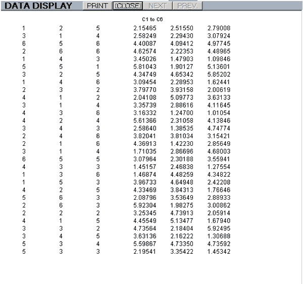
A screen display has buttons to select the NEXT and PREVious pages, when applicable, and a PRINT button.
If the data can be identified as integer it is displayed with no decimal points. Otherwise, it is rounded to 4 d.p. no matter how many places there are.
The maximum size of a display page is 53 rows of 7 columns.
value(object name)
This will display on the screen the current value of the object concerned which can be a program variable or an element of data using the st[row:column] notation.
e.g. value(pp[2]) will display the current value of the second element of the pp[ ] array.
histogram(dimensions,type,steps,first column number,last column number)
This will display on the screen histograms of the data in the selected columns.
The acceptable values for the first two parameters are:-
| Dimensions | |
| Values | Result |
| 2D | A two dimensional display |
| 3D | A three dimensional display |
| Type | |
| Values | Result |
| hist | Histogram |
| p_d_f | Probability density function |
| c_d_f | Cumulative distribution function |
e.g. histogram(2D,hist,6,1,3) will display a 2-dimensional histogram with three sets of bars representing the data in columns 1 to 3, split into 6 steps.
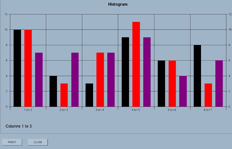
The display has a PRINT and CLOSE button.
N.B.3D displays can be rotated around their axes by holding down the CTRL key, left-clicking the mouse and dragging.
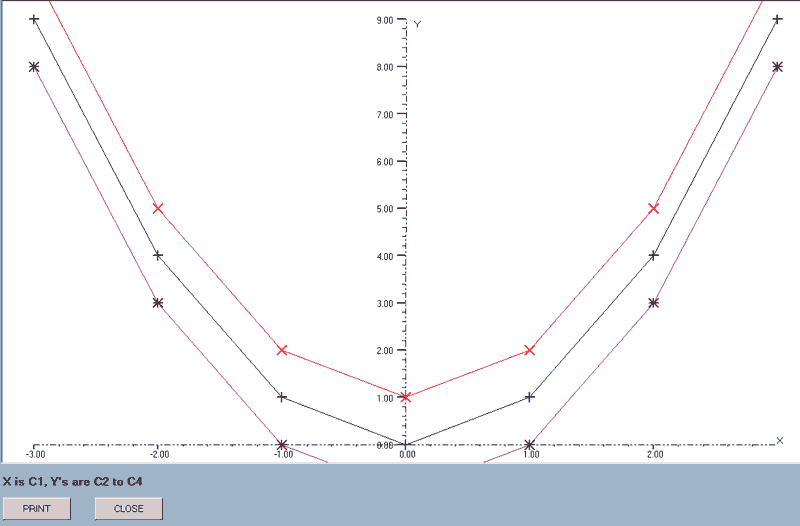
point_plot(axes,first column number,last column number)
This will display on the screen scattergrams of the data in the columns concerned.
e.g. point_plot(axes,1,3) will display scattergrams of the data in columns 1 to 3.
The 'axes' parameter, (axes or no_axes), defines whether axes are to be drawn for this plot.
Essentially, this allows you to overlay several sets of data by selecting 'axes' for an initial plot and then 'no_axes' for a subsequent plot or plots.
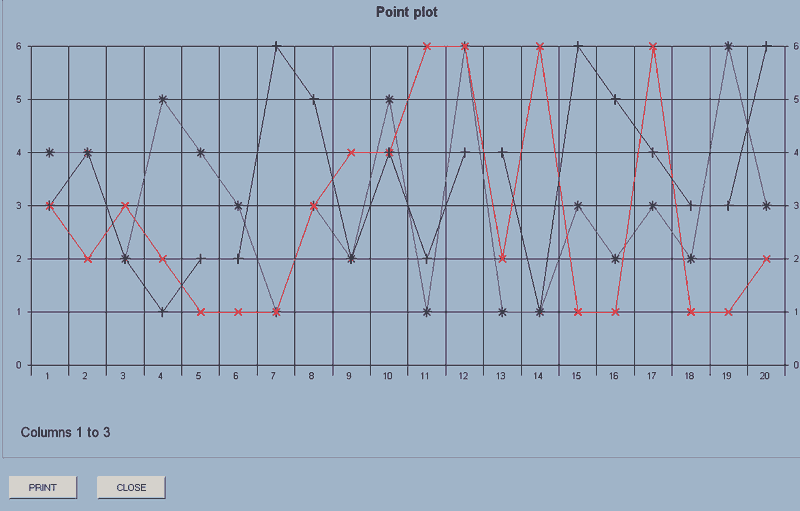
If you then use point_plot(no_axes,6,7), the plots for the data in columns 6 and 7 will be added to the display.
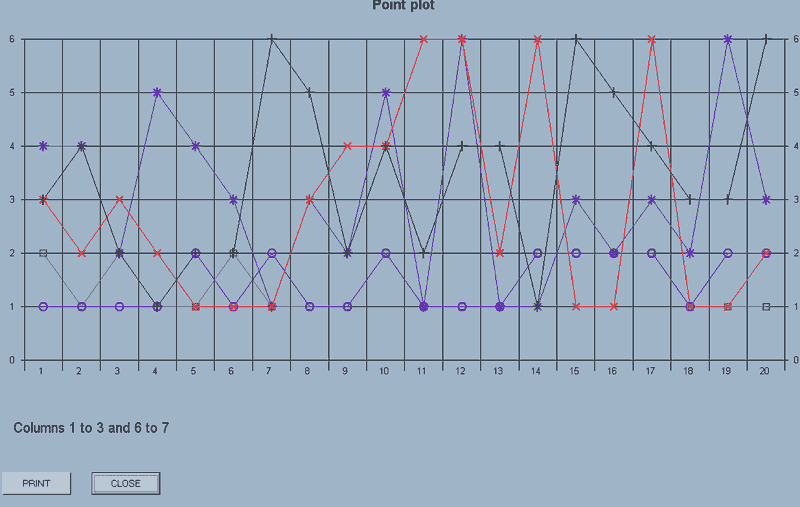
The display has a PRINT and CLOSE button.
Each set of data is plotted using a different symbol up to the maximum of 8 sets of data.

The maximum number of points which will be displayed is 30. If there are more than this in a selected column, a sample is taken rather than having an error message displayed.
If there are different number of points in a block of columns, it's the first column which is used to set the number for display.
graph(axes,markers,x-data column number,first y_data column number,last y_axis column number)
The data in the x-axis column is plotted against that of each of the columns in the block of y-axis data.
e.g. graph(axes,markers,1,2,4) will draw graphs with point markers, where the X-data is that in column 1 and there are three graphs corresponding to Y-data in columns 2 to 4.
The acceptable values for the first two parameters are:-
| Axes | |
| Values | Result |
| axes | Axes are added to a new graph |
| no_axes | Subsequent plots are added to an existing graph. |
| Markers | |
| Values | Result |
| markers | Points are emphasised with the same markers used for 'point_plot' |
| no_markers | No markers are used. |
The axes ranges are calculated from the X-data column and the first of the Y-data columns. The actual range is rationalised to give ranges in simple numbers and the axes do not pass through the origin if this is not within the range of the data.
The X-data column can be included within the block but will be skipped as the graphs are drawn. e.g. graph(axes,markers,3,1,6) is acceptable: column 3 provides the X-data and graphs will be drawn using columns 1, 2, 4, 5 and 6 as the Y-data.
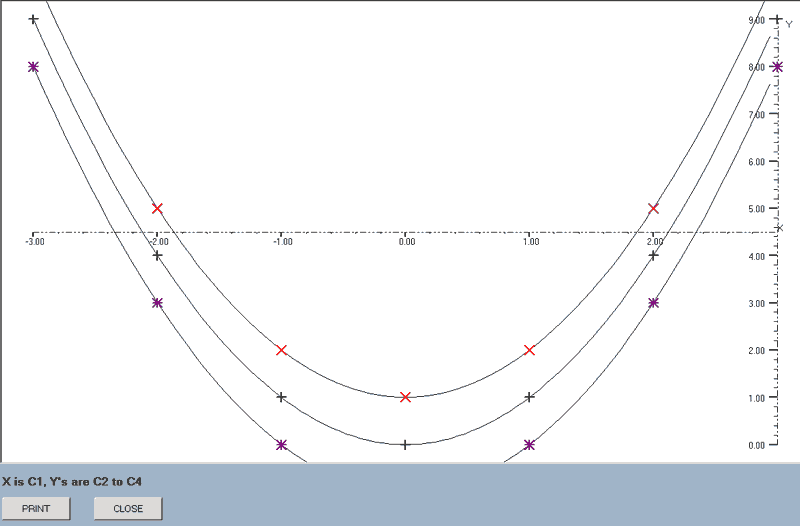
best_line(axes,type,x-data column number,first y_data column number,last y_data column number)
This will find the best line that fits the sets of data: the data in the x-axis column being plotted against that of the block of y-axis data.
e.g. best_line(axes,quad,1,2,4) will draw the best quadratics for the data sets where the X-data is that in column 1 and there are three graphs corresponding to Y-data in columns 2 to 4.
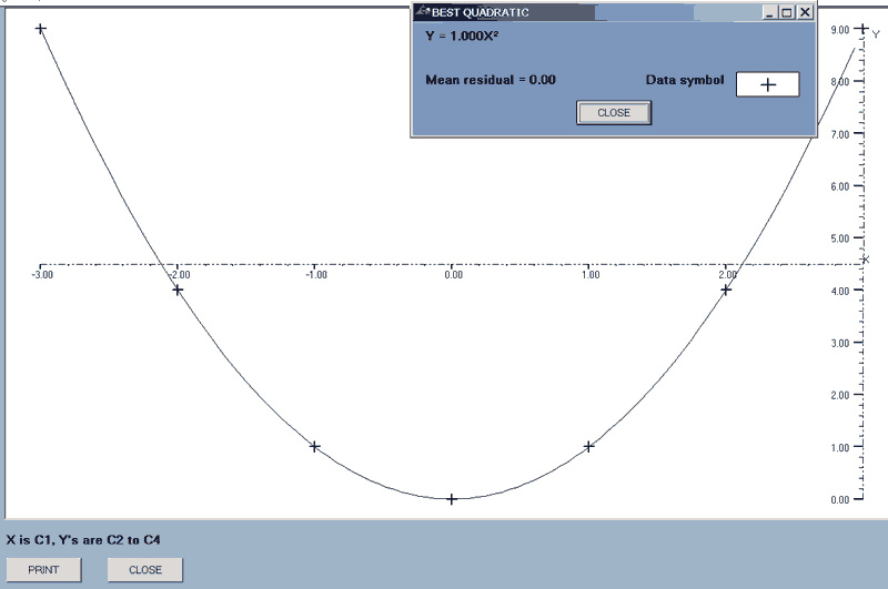
After each line is drawn, there is a display of the equation of the line concerned, the mean relative residual, (MRR), and the symbol used for the data points.
Each residual = data - function value and the MRR is defined as
Σ(absolute residuals)/Σ(absolute data).
The acceptable values for the first two parameters are:-
| Axes | |
| Values | Result |
| axes | Axes are added to a new graph |
| no_axes | Subsequent plots are added to an existing graph. |
| Type | |
| Values | Result |
| linear | The best straight line is found. |
| quad | The best quadratic is found. |
| ab^x | The best line of the form y = a(bx) is found. |
| ax^r | The best line of the form y = a(xr) is found. |
The X-data column can be included within the block but will be skipped as the graphs are drawn. e.g. best_line(axes,linear,2,1,4) is acceptable: column 2 provides the X-data and graphs will be drawn using columns 1, 3 and 4 as the Y-data.
find_line(x-data column number,y_data column number)
This plots all of the available lines of best-fit for the data in the specified columns.
The mean relative residual for each line is stored and, if the graphs are printed, this information is added to the display as described above for the 'best_line' command and the minimum M.R.R. is listed as an aid in deciding which is the best line for this data.
A check is made at the start to see if the X or Y ranges include zeroes and, if they do, the two power graphs, y = a(bx) and y = a(xr), are excluded.
The first marker,
 , is used for the data and each line is drawn in a different colour.
e.g. find_line(1,2) will draw the four lines for the data in columns 1 and 2.
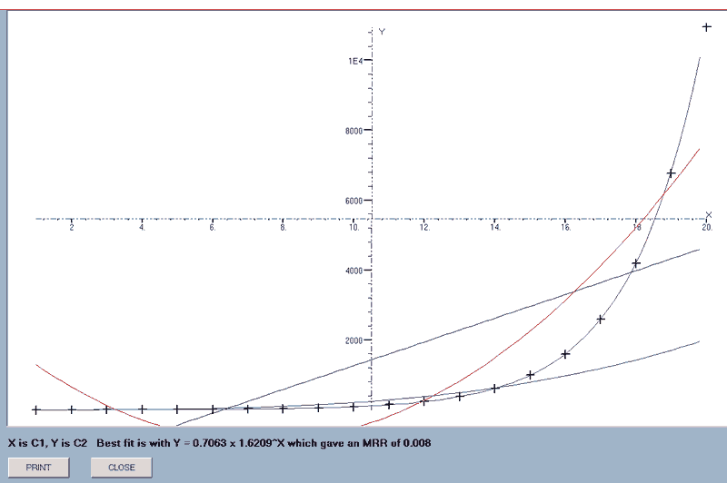
When all the graphs have been drawn, the equation of the one giving the smallest MRR is appended to the data display which, in this case, is the Fibonacci series!